![]()
 |
EVIDENCE ON FACTORS THAT INFLUENCE THE PROBABILITY OF A GOOD PERFORMANCE IN THE PRINCIPLES OF ECONOMICS COURSE |
 |
by Larry V. Ellis, Garey C. Durden, and Patricia E. Gaynor
Larry V. Ellis is an Associate Professor of Economics, and Garey C. Durden and Patricia E. Gaynor are Professors of Economics at Appalachian State University.
If you do not like the background color, you can change it by highlighting the color you prefer in the scroll box below.
Introduction
How important is class attendance for student performance in university level economics courses, other things being equal? The somewhat sparse evidence on this question is mixed. An early study by McConnell and Lamphear (1969) found no significant difference in the performances of students who did and did not attend class. Paden and Moyer (1969) found that class attendance was important only when non-standardized tests were used. Buckles and McMahon (1971) reported that when classes only explained material covered in reading assignments, attendance did not improve student understanding of economics. A paper by Browne, et al. (1991) concluded that students who did not attend a typically structured microeconomic principles class with lectures did just as well on the Test of Understanding College Economics (TUCE) as those who did.
There is also an increasing body of work which suggests that attendance does affect performance. Schmidt (1983), for example, reported that time spent attending lectures in a macroeconomic principles course contributed positively to performance. More recently, Park and Kerr (1990) found that attendance was a determinant of student performance in a money and banking course, although it was not as important as a student's GPA and percentile rank on a college entrance exam. In a widely cited study, Romer (1993) found that attendance did contribute significantly to the academic performance of students in a large intermediate macroeconomics course. For a sample of students enrolled in agricultural economics and agribusiness courses, Devadoss and Foltz (1995) were able to report that the more classes attended, the better the students' grades. Finally, Durden and Ellis (1995) found that student absences had a significant, negative effect on student performance in the principles of economics course.
When there is a lack of consensus in the literature on an issue such as this one, further empirical work is usually necessary. It is often useful in such work to employ a methodology different from those in prior studies. This not only provides a fresh perspective, but it also increases confidence in a study's results when those results confirm the findings of prior work. Our objective in undertaking this study was to provide additional evidence on the relationship between class attendance and student performance in the principles of economics course.
The method we employ to examine this relationship differs from that of previous studies in that we treat student performance as a dichotomous variable. In other words, we view the student as either having done well or having done poorly in the course. This permits us to use a logit model to examine student performance and how it is influenced by various factors. As a result, we are not only able to confirm some of the findings of previous work, but we are also able to uncover some subtle relationships not revealed by other methods. The following section of this paper describes the model we used. This is followed by a description of the data, a discussion of the empirical results and, finally, some conclusions.
THE CONCEPTUAL FRAMEWORK
Our intuition and anecdotal experience tell us that a student's chances of performing well in principles of economics are improved with good attendance, while a student's odds of not doing well are increased by poor attendance. To test these hypotheses we use a logit model based on the cumulative logistic probability function and specified as:
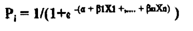 |
(1) |
where Pi is the probability of a particular outcome, a is a constant term and b1,. . .,bn are estimated coefficients on the independent variables, X1,. . .,Xn, hypothesized to affect the outcome.
In logarithmic form, equation (1) can be written as,
| Log (Pi /1-Pi) = a + b1C1 + ,...,+ bnCn .............................................................. | (2) |
which serves as our regression model. The dependent variable in the regression model is simply the logarithm of the odds that a particular outcome will occur.
An important purpose of the logit model is that it transforms the problem of predicting probabilities within a (0,1) interval to the problem of predicting the probability of an events occurring within the range of the entire real line [Pindyck and Rubinfeld. 1991]. When dealing with a dichotomous dependent variable (as in our case), there is a close similarity between the logit and probit models. Thus, it does not matter much (unless the data is heavily concentrated in the tails of the function) which one is used. Since the logit function represents a close approximation to the cumulative normal and is simpler to work with, we chose it. [Kmenta, 1986].
THE DATA
The data for this study were collected by surveying students at the end of the semester in several sections of the principles of economics course (both micro and macro). A questionnaire was administered over five semesters: Spring and Fall 1993, Spring and Fall 1994, and Spring 1995. The data on absences are the estimated number of classes missed during the semester as reported by the students themselves.1 The observations on student grades are simply the percentage of possible course points earned by the student for the semester.
EMPIRICAL RESULTS
The regression model of equation (2) may be written in final, operational form as,
| Log (Pi /1-Pi) = a + b1 ABSENT + b2
RACE + b3 FRATSOR + b4 STATE + b5 HRSCAR + b6 HRSCOMP + b7 GPA + b8HRSWKD + b9 HSCHECON + b10 CALC + b11 SAT + b12 HRSTD ................................................. |
(3) |
where the dependent variable is as defined earlier, and a, b1, b2, etc. are the estimators of the constant term and coefficients on the independent variables, respectively. The set of independent variables is defined in Table 1.
Two versions of equation (3) were estimated. The first version estimates the odds of a student making an A or B (Pi = 1) versus other grades (Pi = 0) when that outcome is affected by the independent variables included in equation (3). The second version of equation (3) estimates the probability of a student making a D or F (Pi = 1) versus other grades (Pi = 0) when that outcome is affected by the same set of independent variables. Because the observations were for individuals and not grouped, the logit model was estimated using a nonlinear maximum-likelihood estimation procedure.
The results from estimating the two versions of equation (3) are reported in Table 2. It should be noted that no independent variable set can control for other influences on student performance so that the affect of class absences is perfectly isolated. We feel, however, that the controls represented by the independent variables employed here are sufficient since they include proxies for major influences such as motivation and ability (GPA, SAT) as well as opportunity cost of the student's time (HRSWKD, HRSCAR, HRSTD).
As seen in Table 2, the likelihood of a student making an A or B in principles of economics significantly decreases (at the 5% level) as the number of absences increase; when the student is a member of a fraternity or sorority; and as the number of credit hours carried by the student during the semester increases. On the other hand, the chances of a student making an A or B in the course significantly increases with having taken a calculus course; a higher GPA; and higher SAT scores.2
The coefficient estimates on the second equation reported in Table 2 reveal that the likelihood of making a D or F in principles of economics decreases if the student has a higher GPA; has taken a high school course in economics; or has higher SAT scores. The likelihood of making a D or F in the course significantly increases with the number of absences; when the student is female; and when the student is a member of a fraternity or sorority.
The results reported in Table 2 with respect to the direction and significance of the effects of the independent variables conform very closely to OLS results reported in an earlier study [Durden and Ellis, 1995] with one important exception that is discussed below. Given the very different statistical methodology employed here, the similarity of the results in the two studies justifies an increased confidence in conclusions based on these results.
The approach employed here also allows further insight into the nature of the influence of certain variables on student performance in principles of economics courses. In our earlier study, we found that having taken a high school economics course improves performance in the college course. The estimates on HSCHECON in Table 2 show that having taken such a course does not improve the likelihood of getting an A or B in the college course, but it does significantly reduce the odds of getting a D or F. In other words, other things being constant, a high school economics course appears to help the poorer students, but it is not a factor in the performance of better students.3
A similar asymmetry characterizes the GENDER variable. In our earlier study, we found no significant difference in the performance of males and females. Although this is contrary to much of the evidence in the literature (See Siegfried, 1979 and Lumsden and Scott, 1987.), it is consistent with a recent study [Williams, et al., 1992] that also found that gender differences were not significant in student performance. In Table 2, the coefficient on GENDER is negative in both the GRADE A or B and the GRADE D or F equations. This indicates a greater likelihood of females falling into the two grade ranges. But since the coefficient is not significantly different from zero in the A or B equation, there is no difference between males and females in the probability of getting an A or B. Given that the GENDER variable is both negative and significant in the D or F equation, however, the chance of making a D or F is greater for females than for males.
The relationship between attendance and performance was further explored with special emphasis on the gender difference just noted. The GRADE A or B equation was estimated for females only, males only, and for all students combined. The same was done with the GRADE D or F equation. The results for females only and males only are reported in Table 3.4 The values reported in Table 4 were obtained by calculating the right hand side of the appropriate equation from Table 3 for zero to nine absences using the mean values for the other independent variables. The antilog of this result was then used to find the actual probability estimates.5
As can be seen in Table 4, the probability of making an A or B decreases as the number of absences increases. This is true for both males and females as well as all students combined. The results indicate that a typical student with no absences has about a one in five chance of making an A or B. With four absences, however, the odds of making a good grade drop to one in eight. It is also apparent from Table 4 that the probability of making an A or B for any given number of absences is greater for females than for males. The results reported earlier from Table 2, however, suggest that this difference is probably not significant.
The values shown in Table 5 are the probabilities of making a D or F for absences ranging from zero to nine and were calculated in the same manner as those in Table 4. The odds of making a D or F increase as absences increase for males, females and all students combined. It is also evident that the probability of a female getting a D or F for any given number of absences is greater than for a male. The significance of the coefficient estimate on the GENDER variable in the estimates reported in Table 2 (the GRADEDF equation) suggests that this difference in males and females is probably significant.
CONCLUSIONS
The logit analysis employed here reveals that the probability of a student earning a grade of A or B in a principles of economics declines as the number of missed classes increases, and the probability of a student earning a D or F increases as classes missed increases. Other factors that positively affect the chances of earning a good grade are the student's GPA, taking calculus and SAT scores. Other negative influences include membership in a fraternity or sorority and the number of credit hours carried during the semester.
In addition to poor attendance, the odds of receiving a poor grade in a principles of economics course are increased by membership in a fraternity or sorority and being female. There's less chance of a low grade for those students with higher GPAs; those that have taken a course in high school economics and those with higher SAT scores.
Our previous finding, based on OLS regressions, that no difference exists in the performance of males and females in principles of economics no longer holds. The logit analysis employed in this study indicates that while females are just as likely as males to do well in principles, they are more likely than males to do poorly. This is true for virtually all levels of class attendance, other things being held constant.
NOTES
1. Since some classes were large, roll was not called in all sections. However, one researcher was able to correlate attendance on eight unannounced quizzes with student-reported absences. The correlation was 0.79 (p < 0.01) even though some students reported more than eight absences.
2. The interpretation of the individual estimated parameters must be done with care, since the left side of the equation is the logarithm of the probability of a particular outcome, not the actual probability. For example, a one unit change in a student's GPA will lead to a .019 increase in the logarithm of the odds that a student will make an A or B in the course.
3. It is tempting to speculate that this may be because the better students don't take high school economics. In North Carolina, where this study was conducted, however, all students are required to take a course with economics content at the ninth grade level. Almost ninety percent of those in our student sample are from North Carolina.
4. The results in Table 3 suggest that the negative influence of fraternity and sorority membership on student performance may occur primarily through females. This also appears to be the case for the effect of a high school economics course in reducing the odds of obtaining a grade of D or F.
5. It should be noted that in Tables 4 and 5 the probabilities reported for "All Students" will not fall in between those for "Females" and "Males" and represent a kind of weighted average of their probabilities. This is because the logit equation for "All Students" used to calculate these probabilities included a dummy variable for gender where the other two equations did not. Also, the weights for the respective variables are different for each of the three equations.
DESCRIPTION OF VARIABLES
(Number of observations = 634)
| Variable | Mean | Std. Dev. | Variable Description |
| GRADE-AB GRADE-DF ABSENT SAT GPA HISCHEC CALC RACE FRATSOR HRSCOMP GENDER HRSTD HRSCAR HRSWKD STATE |
3.464 970.145 270.470 0.473 0.625 0.945 0.197 46.210 0.609 10.490 13.816 8.229 0.894 |
3.624 164.211 56.200 0.500 0.485 0.229 0.398 24.969 0.488 7.351 4.661 11.336 0.308 |
1 if student's percentage of
possible course points is 80% or above, 0 otherwise. 1 if student's percentage of possible course points is 65% or less, 0 otherwise. Number of absences. SAT score (combined math and verbal) Grade point average (x 100) on a four point scale 1 if had high school economics, 0 otherwise 1 if taken college calculus, 0 otherwise 1 if white, 0 if African American, Hispanic, etc. 1 if sorority or fraternity member, 0 otherwise Total credit hours completed prior to current semester 1 if male, 0 if female Time spent studying (hours per week) Number of credit hours carried during current semester Number of hours worked per week in job 1 if North Carolina, 0 otherwise |
LIKELIHOOD OF STUDENTS ACHIEVING A GOOD OR BAD GRADE
LOGIT ANALYSIS
| Independent Variable | Grade A OR B | Grade D OR F | ||
| Coefficient | T-value | Coefficient | T-value | |
| CONSTANT | -10.083 | -8.197** | 8.078 | 7.235** |
| ABSENT | -0.132 | -3.496** | 0.130 | 4.420** |
| GENDER | -0.069 | -0.306 | -0.566 | -2.685** |
| RACE | 0.348 | 0.646 | -0.745 | 01.720^ |
| FRATSOR | -0652 | -2.317* | 0.554 | 2.249* |
| STATE | -0.572 | -1.653^ | 0.129 | 0.384 |
| HRSCAR | -0.046 | -1.979* | 0.004 | 0.161 |
| HRSCOMP | 0.001 | 0.189 | -0.002 | -0.454 |
| GPA | 0.019 | 8.139** | -0.015 | -6.740** |
| HRSWKD | -0.014 | -1.353 | 0.001 | 0.122 |
| HSCHECON | 0.121 | 0.554 | -0.602 | -2.957** |
| CALC | 0.777 | 3.224** | -0.246 | -1.177 |
| SAT | 0.004 | 4.996** | -0.004 | -4.900 |
| HRSTD | 0.016 | 1.122 | -0.019 | -1.281 |
| LOG LIKELIHOOD | -267.728 | -304.076 | ||
| N | 634 | 634 | ||
** Statistically significant at 1% level
* Statistically significant at 5% level
^ Statistically significant at 10% level
LIKELIHOOD OF A PARTICULAR GRADE: FEMALES VS. MALES
LOGIT ANALYSIS
| INDEPENDENT VARIABLE | GRADE A OR B | GRADE D OR F | ||||||
| FEMALES | MALES | FEMALES | MALES | |||||
| Coefficient | T-value | Coefficient | T-value | Coefficient | T-value | Coefficient | T-value | |
| CONSTANT | -9.588 | -4.668** | -10.984 | -6.676** | 7.779 | 4.058** | 7.753 | 5.498** |
| ABSENT | -0.146 | -2.133* | -0.125 | -2.667** | 0.151 | 2.761** | 0.129 | 3.565** |
| RACE | 0.261 | 0.317 | 0.501 | 0.595 | -1.076 | -1.438 | -0.599 | -1.056 |
| FRATSOR | -0.763 | -1.674^ | - 0.409 | -1.101 | 1.038 | 2.653** | 0.103 | 0.300 |
| STATE | -1.725 | -2.707** | 0.146 | 0.317 | 1.178 | 1.658^ | -0.377 | -0.942 |
| HRSCAR | -0.053 | -1.018 | - 0.049 | -1.777^ | -0.027 | -0.573 | 0.011 | 0.397 |
| HRSCOMP | -0.009 | -1.085 | 0.006 | 1.090 | -0.000 | -0.043 | -0.005 | -0.934 |
| GPA | 0.026 | 5.672** | 0.016 | 5.700** | -0.017 | -4.639** | -0.013 | -4.522** |
| HRSWKD | -0.010 | -0.531 | - 0.024 | -1.810^ | -0.017 | -1.043 | 0.012 | 1.061 |
| HSCHECON | -0.005 | -0.014 | 0.150 | 0.534 | -0.891 | -2.527** | -0.404 | -1.543 |
| CALC | 0.695 | 1.722^ | 0.740 | 2.388* | -0.227 | -0.653 | -0.282 | -1.127 |
| SAT | 0.004 | 2.745** | 0.005 | 4.114** | -0.004 | -2.504** | -0.005 | -4.159** |
| HRSTD | -0.021 | -0.801 | 0.030 | 1.691^ | -0.023 | -0.837 | -0.022 | -1.157 |
| Log Likelihood | -96.281 | -163.838 | -112.426 | -184.798 | ||||
| N | 248 | 386 | 248 | 386 | ||||
** Statistically significant at 1% level
* Statistically significant at 5% level
^ Statistically significant at 10% level
PROBABILITIES OF MAKING AND "A" OR "B"FOR A SELECTED NUMBER OF ABSENCES
NUMBER OF ABSENCES |
||||||||||
| 0 | 1 | 2 | 3 | 4 | 5 | 6 | 7 | 8 | 9 | |
| All Students | .195 | .175 | .157 | .140 | .125 | .112 | .099 | .088 | .078 | .069 |
| Females | .286 | .257 | .230 | .205 | .182 | .162 | .143 | .126 | .111 | .097 |
| Males | .244 | .222 | .201 | .182 | .164 | .147 | .132 | .119 | .106 | .095 |
PROBABILITIES OF MAKING A "D" OR "F" FOR A SELECTED NUMBER OF ABSENCES
NUMBER OF ABSENCES |
||||||||||
| 0 | 1 | 2 | 3 | 4 | 5 | 6 | 7 | 8 | 9 | |
| All Students | .237 | .261 | .287 | .314 | .343 | .373 | .404 | .435 | .468 | .500 |
| Females | .129 | .147 | .167 | .189 | .213 | .239 | .268 | .299 | .331 | .365 |
| Males | .120 | .134 | .150 | .167 | .186 | .206 | .228 | .251 | .276 | .303 |
REFERENCES
Brasfield, David, Danny Harrison and James McCoy. "The Impact of High School Economics on the College Principles of Economics Course." Journal of Economic Education, Spring 1993, 24(2), pp. 99-111.
Brasfield, David, James McCoy and Martin Milkman. "The Effect of University Math on Student Performance in Principles of Economics." Journal of Research and Development in Education, Summer 1992, 25(4), pp. 240-47.
Brauer, Jurgen, et. Al. "Correspondence." Journal of Economic Perspectives, Summer 1994, 8(3), pp. 205-215.
Browne, Neil M., John Hoag, Mark V. Wheeler, and Nancy Boudreau. "The Impact of Teachers in Economic Classrooms." Journal of Economics, 1991, XVII, pp. 25-30.
Buckles, Stephen G. and M.E. McMahon. "Further Evidence on the Value of Lecture in Elementary Economics." Journal of Economic Education, Spring 1971, 2(2), pp. 138-41.
Devadoss, Stephen, and John Foltz. 1995. "Evaluation of Factors Influencing Student Class Attendance and Performance". Manuscript.
Durden, Garey C. and Larry V. Ellis. "The Effects of Attendance on Student Learning in Principles of Economics." American Economic Review Papers and Proceedings, May, 1995, 85(2), pp. 343-346.
Kmenta, Jan. 1986. Elements of Econometrics. 2nd ed. New York: Macmillan.
Lumsden, Keith G. and Alex Scott. "The Economics Student Reexamined: Male-Female Differences in Comprehension." Journal of Economic Education, Fall 1987, 18(4), pp. 365-375.
McConnell, Campbell R. and C. Lamphear. "Teaching Principles of Economics Without Lectures." Journal of Economic Education, Fall 1969, 1(4), pp. 20-32.
Myatt, A. and C. Waddell. "An Approach to Testing the Effectiveness of the Teaching and Learning of Economics at High School." Journal of Economic Education, Summer 1990, 21(3). Pp. 355-63.
Paden, Donald W. and M. Eugene Moyer. 1969. "The Effectiveness of Teaching Methods: The Relative Effectiveness of Three Methods of Teaching Principles of Economics." Journal of Economic Education, 1 (Fall), pp. 33-45.
Park, Kang H. and Peter M. Kerr. ADeterminants of Academic Performance: A"Multinomial Logit Approach." Journal of Economic Education, Spring 1990, 21(2), pp. 101-11.
Pindyck, R.S. and D.L. Rubinfled. 1991. "Econometric Models and Economic Forecasts." 3rd ed. New York: McGraw-Hill.
Romer, David. "Do Students Go to Class? Should They?" Journal of Economic Perspectives, Summer 1993, 7(2), pp. 167-74.
Schmidt, Robert M. "Who Maximizes What? A Study in Student Time Allocation." American Economic Review, May 1983, 73(2), pp. 23-28.
Siegfried, John J. and Rendigs Fels. "Research on Teaching College Economics: A Survey." Journal of Economic Literature, September 1979, 17(3), pp. 923-969.
Williams, Mary L., Charles Waldauer and Vijaya G. Duggal. "Gender Differences in Economic Knowledge: An Extension of the Analysis." Journal of Economic Education, Summer 1992, 23(3), pp. 219-31.