If markets are efficient in semi

Earnings Surprises and Stock Returns: Some Evidence from Asia/Pacific and Europe

by H. Christine Hsu

H. Christine Hsu CHSU@csuchico.edu is a Professor of Finance in the Department of Finance and Marketing, College of Business, California State University, Chico.

The study reported on in this article suggests that the semi-strong form market efficiency appears to be violated in the Asia/Pacific equity market. The findings of this study reveal that the superior (inferior) performance of portfolios is associated with positive (negative) earnings surprises, and that portfolio returns increase with earnings surprises over the years of 1995-1999 in this international equity market. Regression results suggest that the earnings surprises are much more powerful in predicting portfolio returns than they are in predicting stock returns. The author concludes from the study that portfolio earnings surprises information is useful in predicting one-year ahead portfolio returns and that a trading strategy based on earnings surprises earns abnormally high returns year after year. Needless to say, this study has significant implications for investors / portfolio managers in making their asset allocation decisions in Asia/Pacific equity market.

If markets are efficient in semi-strong form as defined in Fama (1970), then stock prices will adjust immediately to public information such as the release of street consensus earnings estimates and the announcement of actual earnings. As a result, a trading strategy based on publicly available earnings information cannot be profitable. Evidence from recent studies suggests market inefficiency in semi-strong form. For example, Charitou and Panagiotides (1999) find that an earnings-based trading strategy earns higher excess returns than a cash flow-based trading strategy in the U.K.; Bagoli, Beneish and Watts (1999) conclude that trading strategies based in the relation between Whisper and First Call earnings forecasts earn abnormal stock returns; Alexander and Ang (1998) demonstrate that the U.S. equity markets do respond to earnings paths; Cheung, Chung and Kim (1997) show that trading strategies based on earnings to price ratio of a sample of Hong Kong firms yield significant excess returns for various holding periods up to two years; and Bernard and Thomas (1990) find that part of the stock price response to this quarter's earnings announcement is predictable from earnings one to four quarters back. The objectives of this study are to add one more piece of evidence to support the hypothesis of semi-strong form market inefficiency and to investigate whether earnings surprises can be used to create a profitable trading strategy that captures stocks with superior performance.

DATA AND METHODOLOGY

Earnings expectations data on more than 18,000 international stocks from 1987 through 2000 are available in Institutional Brokers Estimate Systems (I/B/E/S) historical summary database. [1] Since data on many firms in the emerging markets became available in 1993 or later, my sample period runs from 1994:12 through 1999:12. The universe of firms is composed of international firms in 40 countries from Asia/Pacific and Europe. To be included in the sample, the common stock of an international firm must have common shares outstanding (at least one billion shares), price (at least $5) [2] actual earnings per share, consensus earnings per share estimate, and standard deviation of earnings estimates data in December of year t, and dividend and stock price data in December of year t+1. I define consensus earnings per share estimate as the mean forecasted earnings per share when there are at least three financial analysts contributing to I/B/E/S estimates. The minimum common shares outstanding and price screening standards are employed to ensure that only firms with big market capitalization (= price x common shares outstanding) are included in the analysis. I use the standardized unexpected earnings (SUE) to measure the earnings surprises. It is defined as

SUE_t = (A_t - F_t) / SD_t

Where SUE_t = year t standardized unexpected earnings

A_t = year t actual earnings per share reported by the firm

F_t = year t consensus earnings per share forecasted by analysts in year t-1

SD_t = year t standard deviation of earnings estimates

SUE measures the deviation of actual earnings from the mean forecasted earnings scaled by its standard deviation. If financial analysts over-forecast, then there is negative earnings surprise (SUE <0), and vice versa. The absolute value of SUE is a direct indicator of the degree of the earnings surprises (or the forecasting errors). To examine the relation between the earnings surprise and stock performance, I rank the stocks in terms of SUE at the end of each year t, and compute their rates of return in year t+1. The rate of return is calculated as the sum of the stock's dividend yield and capital gains yield,

R_t+1 = [DIV_t+1 / P_t ]+ [(P_t+1- P_t) / P_t ]

Where R_t+1 = year t+1 rate of return

DIV_t+1 = year t+1 dividends on common stock

P_t+1 = year t+1 price of stock

P_t = year t price of stock

To eliminate outliers in the analysis, I exclude five percent of the stocks with the highest SUE and five percent of the stocks with the lowest SUE from the sample. This yields 11,258 stock-year observations during the sample period, where 243 observations have no earnings surprises (SUE = 0). Since the focus is on the association of earnings surprises with stock returns, these zero SUE observations are excluded from the sample. This results in 11,015 stock-year observations for the study, 2021 observations from Asia/Pacific equity market, and 8994 observations from Europe equity market.

To investigate whether stock behavior is affected differently by the direction of earnings surprises, I then group the stocks into two portfolios based on the sign of SUE. Portfolio A consists of the stocks with positive earnings surprises (SUE > 0), and Portfolio B with negative earnings surprises (SUE < 0). Table 1 contains the descriptive statistics of common shares outstanding, SUE and portfolio returns of the base sample over the study period. Table 2 contains the descriptive statistics of the base sample by year. Table 3 summarizes the difference between the two portfolios’ mean returns by year.

To evaluate how the earnings surprise in year t (SUE_t) is associated with the stock return in year t+1 (R_t+1) statistically, I run the following regression in each market for the stocks in each of the two portfolios, namely, Portfolios A and B.

R_t+1= a + b SUE_t+ e

Where a = the intercept of the regression line

b = the sensitivity of stock return to SUE

e = stock return movement that is uncorrelated to SUE

If the earnings surprises coefficient b is significantly different from zero, then the association between SUE and the stock return is not due to chance. If coefficient b is positive (negative), then there is a direct (inverse) relation between SUE and stock return. Table 4 summarizes the regression results for the stocks in each of the two portfolios (Portfolios A and B) by market.

To examine how positive earnings surprises affect portfolio performance in Asia/Pacific market, I assign stocks in Portfolio A into one of the twenty subgroups (Asia/Pacific Portfolios A1-A20) on the basis of their SUE annually. That is, at the end of each year from 1994 through 1998 in Asia/Pacific market, five percent of the stocks with the highest SUE are assigned to Asia/Pacific Portfolio A1, five percent of the stocks with the next highest SUE are assigned to Asia/Pacific Portfolio A2, and so on. Table 5 contains the descriptive statistics of the twenty portfolios with positive earnings surprises in Asia/Pacific market. The same grouping procedure is employed for the stocks with negative SUE in Asia/Pacific market. Table 6 contain the descriptive statistics of the twenty portfolios with negative earnings surprises in Asia/Pacific market (Asia/Pacific Portfolios B1-B20).Portfolio B1 consists of five percent of the stocks with the lowest negative earnings surprises and Portfolio B20 consists of 5% of the stocks with the highest negative earnings surprises. To examine how earnings surprises affect portfolio returns in Europe market, I adopt the same grouping procedures and constructed twenty portfolios with positive SUE (Europe Portfolios A1-A20) and twenty portfolios with negative SUE (Europe Portfolios B1-B20). [3]

To investigate whether the relationship between portfolio performance in year t+1 and portfolio earnings surprises in year t is statistically significant, I finally regress the portfolio return against the portfolio SUE for Portfolios A1-A20 and Portfolios B1-B20 in each market. Table 7 provides the regression results for the portfolios by market.

RESULTS AND IMPLICATIONS

Table 1 shows there were 4,522 observations with positive earnings surprises (or under-forecast errors) and 6,493 with negative surprises (or over-forecast errors) during the 1994-1998 sample period in the international equity markets. (Click here to go to the tables.) It appears that financial analysts were not very accurate in forecasting earnings and that they tend to over-forecast more often than to under-forecast earnings of stocks over the five years ending in December 1998. This is found not only in Asia/Pacific market but in the European market as well. Table 2 confirms the analysts' tendency to over-forecast earnings in all five years (1994-1998) covered in this study. The evidence of over-forecasting is the strongest in 1998, during which there were 1,522 stocks with negative earnings surprises and only 591 stocks with positive earnings surprises in the markets. This evidence supports the findings from prior studies that analysts are inefficient in predicting earnings per share and that they tend to over-forecast earnings of the stocks (Butler and Lang (1991), Brous and Kini (1993), Kang, O'Brien and Sivaramakrishnan (1994), Dreman and Berry (1995), Olsen (1996), Hunton and McEwen (1997), Chopra (1998), and Easterwood and Nutt (1999)). This upward biased earnings estimation may be attributable to economic incentives to promote the purchase of the stocks as a result of the fact that the analysts are employed by brokerage or investment banking firms (Brown (1993), Dugar and Nathan (1995), Carleton, Chen and Steiner (1998), Lin and McNichols (1998), and Hayes (1998)). Or it may be attributable to the pressure to present favorable earnings forecasts because the analysts need to maintain, if not enhance, access to the firms they follow (Schipper (1991), Pratt (1993), Francis and Philbrick (1993), Clayman and Schwartz (1994), and Das, Levine and Sivaramakrishnan (1998)).

Table 1 also shows that on an annual basis, Portfolio A outperformed Portfolio B in terms of mean return (75.4% vs. 39.7%) and median return (13.4% vs. –3.7%) over the five years, 1995 through 1999 inclusive. (Click here to go to the tables.) One might wonder if Portfolio A's excess return is due to risk. The answer is no. In fact, Portfolio A's variability in return (standard deviation) is lower than that of Portfolio B (1.578 vs. 1.648). Table 1 suggests that the portfolio with positive earnings surprises (Portfolio A) had higher return and lower risk as compared to the portfolio with negative earnings surprises (Portfolio B) in both the Asia/Pacific and Europe markets. It appears that the positive (negative) earnings surprise is good (bad) news to investors/portfolio managers in these international equity markets.

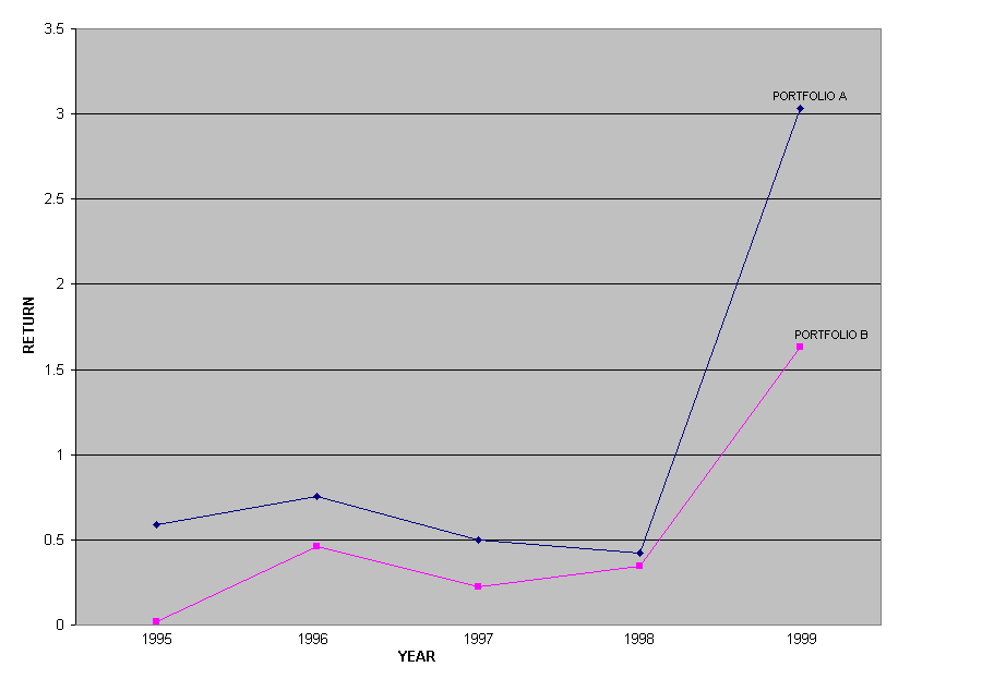
If the markets are efficient in semi-strong form, then the abnormal returns of Portfolio A should disappear immediately after the earnings surprises information is factored in stock prices, and a SUE based trading strategy cannot be profitable year after year. Table 2 suggests otherwise; the portfolios with positive earnings surprises outperformed those with negative earnings surprises in every single year from 1995 to 1999 in the international equity markets. (Click here to go to the tables.) The results are graphed in Figures 1, 2 and 3, where the mean returns of the stocks in Portfolios A and B are plotted annually in each market. (Click here to go to the figures.) The implication is that arbitrage profits could have been captured if investors/portfolio managers short sold stocks with negative earnings surprises and bought stocks with positive earnings surprises in the international equity markets. That is, at the end of each year from 1994 through 1998, they borrowed shares of the stocks in Portfolio B and sold them; then used the proceeds to invest in the stocks in Portfolio A. They would have lost the return of Portfolio B on the short sales and gained the return of Portfolio A from the long positions over the five-year investment horizon. They could have pocketed an arbitrage return equal to the difference between the two portfolios’ returns in every single year from 1995 to 1999. This trading strategy based entirely on the sign of SUE turned out to be very profitable in Asia/Pacific market as well as in Europe market over the years of 1995 to 1999.

One might argue that the differences between the two portfolios' returns are not statistically significant. As summarized in Table 3, the difference between the two portfolios' mean returns is statistically significant in Asia/Pacific market every single year from 1995 to1999, and it is statistically significant in Europe market in four out of the five years study period. In fact, not only the profit from investing in Portfolio A didn't disappear over time, it became most significant in Asia/Pacific in 1997 and 1999. [4] Asia/Pacific Portfolio A returned a remarkable 81.7% (115.3%) to investors, while Asia/Pacific Portfolio B returned –17.2% (32.4%) in 1997 (1999). (Click here to go to the tables.)

So far the trading strategy is formed on the basis of the sign of SUE. An important question arises: Is there a relationship between the stock return and the size of earnings surprises? Table 4 shows that the coefficient of stock earnings surprises is positive, 0.7117 (0.0997), and significant at the .05 level for stocks in Asia/Pacific Portfolio A and at the .0001 level for stocks in Asia/Pacific Portfolio B, indicating that there is a direct relationship between stock return in year t+1 and its SUE in year t. However, the relationship is very weak, with R-square equal to .0077 (0.0167) for stocks in Portfolio A (Portfolio B). Table 4 also shows that the coefficient of stock earnings surprises is positive for stocks in Europe market, but it is not statistically significant.

The question now becomes: Is there a relationship between portfolio SUE and one-year ahead portfolio returns? According to the regression results in Table 7, SUE in year t has a positive and statistically significant estimated association with the portfolio mean return in year t+1 only in Asia/Pacific market. This relationship is found not only in the portfolios with positive SUE, Asia/Pacific Portfolios A1-A20, (coefficient b = .1633, t-statistics = 2.3456), but in the portfolios with negative SUE, Asia/Pacific Portfolios B1-B20, (coefficient b = .1168, t-statistics = 4.5122). In other words, the portfolio return in year t+1 is an increasing function of its SUE in year t in Asia/Pacific market. That is, portfolio returns increase as SUE values increase, while portfolio returns decline as SUE values decrease. Furthermore, the regression performed for Asia/Pacific Portfolios A1-B20 results in a R-square of .4786, indicating that portfolio SUE in year t contributes significantly towards an explanation of the variation in the portfolio return in year t+1. The results indicate that the use of portfolio SUE information allows better prediction of future portfolio returns than chance would have it in Asia/Pacific equity market. (Click here to go to the tables.)

An important implication is derived. Notice from Tables 5 and 6 that the portfolio with the highest SUE value (Asia/Pacific Portfolio A1) yielded an abnormally high mean return (131.8%), while the portfolio with the lowest SUE value (Asia/Pacific Portfolio B20) yielded an abnormally low mean return (-51.6%). Recognizing the superior (inferior) performance of the portfolio with the highest positive (negative) earnings surprises, investors/portfolio managers could benefit from a one-year holding period trading strategy. Specifically, if they were to reconstruct their portfolios at the end of each year from 1994 to1998 by buying the portfolio with the highest SUE (Asia/Pacific Portfolio A1) and short selling the portfolio with the lowest SUE (Asia/Pacific Portfolio B20), they would have earned an arbitrage return of 183.4% (= 131.8% + 51.6%) over the five years investment horizon.Even if short sale were not allowed in Asia/Pacific market, they could have gained a mean return of 131.8% by investing in Asia/Pacific Portfolio A1 alone.

CONCLUSIONS

This study suggests that the semi-strong form market efficiency appears to be violated in Asia/Pacific equity market. The findings of this study reveal that the superior (inferior) performance of portfolios is associated with positive (negative) earnings surprises, and that the portfolio returns increase with SUE over the years of 1995-1999 in this international equity market. The regression results suggest that the earnings surprises are much more powerful in predicting portfolio returns than they are in predicting stock returns. Based on this study, I conclude that portfolio earnings surprises information is useful in predicting one-year ahead portfolio returns, and that a SUE-based trading strategy earns abnormally high returns year after year. This study demonstrates that investors/portfolio managers could have gained arbitrage returns if they took a long position in the highest SUE portfolio and took a short position in the lowest SUE portfolio at the end of each year from 1994 to 1998. Needless to say, this study has significant implications for investors/portfolio managers in making their asset allocation decisions in Asia/Pacific equity market.

TABLES

TABLE 1: Descriptive Statistics of Common Shares Outstanding, SUE and Portfolio Return of the Base Sample, 1994-1998

	#sh^a	SUE_t	R_t+1	#sh	SUE_t	R_t+1

	Panel I. Both Markets
	Portfolio A			Portfolio B
Mean	741.3	1.391	0.754	678.3	-2.525	0.397
Median	43.4	1	0.134	33	-1.355	-0.037
Standard Deviation	3866	1.269	1.578	3567.4	3.262	1.648
Minimum	1	0.002	-1	1	-21.333	-1
Maximum	69744.7	6.786	35.110	73028.6	-0.002	67.290
Count	4522	4522	4522	6493	6493	6493


	Panel II. Asia/Pacific Market
	Asia/Pacific Portfolio A			Asia/Pacific Portfolio B
Mean	632.5	1.402	1.06	557.3	-3.725	0.198
Median	48.8	0.989	0.068	37.1	-1.912	-0.243
Standard Deviation	2750.2	1.37	1.162	2802.3	4.352	1.295
Minimum	1	0.002	-0.999	1	-21.333	-1
Maximum	43595.7	6.626	35.031	71294.5	-0.013	62.421
Count	671	671	671	1350	1350	1350


	Panel III. Europe Market
	Europe Portfolio A			Europe Portfolio B
Mean	760.3	1.389	0.701	710.1	-2.21	0.45
Median	42.4	1	0.142	31.8	-1.248	0
Standard Deviation	4029	1.25	1.663	3742	2.826	1.682
Minimum	1	0.003	-1	1	-21.065	-1
Maximum	69744.7	6.786	35.110	73028.6	-0.002	67.290
Count	3851	3851	3851	5143	5143	5143

^a. # sh = common shares outstanding in billions of shares

TABLE 2: Descriptive Statistics of Base Sample by Year, 1994-1998

	1994	1994	1995	1995	1995	1996	1996	1996	1997	1997	1997	1998	1998	1998	1999
	#sh	SUE	R	#sh	SUE	R	#sh	SUE	R	#sh	SUE	R	#sh	SUE	R
	Panel I. Both Markets Portfolio A
Mean	565.3	1.406	0.549	644	1.302	0.714	937.6	1.36	0.748	670.2	1.496	0.391	1021.1	1.364	1.84
Median	40.1	1.017	0.024	41.9	0.965	0.202	42.4	1	0.245	45.4	1.059	0.022	50	1	0.393
Standard Deviation	2971.9	1.272	1.528	3598.9	1.172	1.475	4918.9	1.23	1.252	3405.2	1.362	1.079	4499.2	1.285	2.612
Minimum	1	0.007	-1	1	0.003	-0.998	1	0.01	-0.998	1.5	0.004	-0.998	1	0.002	-0.999
Maximum	55417.3	6.226	10.431	49402.2	6.053	4.38	69744.7	5.851	30.043	56733.1	6.625	4.378	63250.4	6.786	35.11
Count	926	926	926	995	995	995	888	888	888	1122	1122	1122	591	591	591
	Panel II. Both Markets Portfolio B
Mean	433.2	-1.827	0.001	572.8	-1.621	0.421	670.6	-1.577	0.179	876.6	-2.207	0.305	812	-4.901	0.886
Median	24.5	-1.208	-0.092	31.6	-1.142	0.065	32	-1.058	0.106	42.2	-1.23	-0.069	37.2	-2.865	-0.368
Standard Deviation	2473.9	1.812	1.562	3100.1	1.586	1.593	3508.3	1.505	1.367	4546.8	2.558	.847	3826.5	5.107	2.773
Minimum	1	-9.154	-1	1	-8.5	-1	1	-7.154	-1	1.5	-14.321	-1	1	-21.333	-1
Maximum	46703.8	-0.01	5.793	56172.1	-0.005	8.264	65534.1	-0.002	14.162	71761.9	-0.01	4.727	73028.6	-0.013	67.29
Count	1087	1087	1087	1578	1578	1578	1106	1106	1106	1200	1200	1200	1522	1522	1522
	Panel III. Asia/Pacific Portfolio A
Mean	195.7	1.48	0.158	276.9	1.444	0.169	394.9	1.61	0.817	592	1.508	0.078	853.1	1.3156	1.153
Median	27.3	1.018	-0.119	39.1	0.851	0.052	74.5	1.303	-0.41	97.1	1.014	-0.115	50	0.9587	0.34
Standard Deviation	397.1	.773	.654	740.8	.767	.509	826.2	1.422	1.217	1603.2	1.514	.692	3565.5	1.2914	2.721
Minimum	1	0.04	-0.998	1	0.035	-0.994	2.3	0.014	-0.88	3.1	0.02	-0.997	1.1	0.0016	-0.999
Maximum	2864.8	6.226	7.598	5323.8	5.597	4.38	5371.9	5.368	27.92	11989.8	6.071	1.096	43595.7	6.626	35.031
Count	84	84	84	70	70	70	78	78	78	64	64	64	375	375	375
	Panel IV. Asia/Pacific Portfolio B
Mean	119.2	-1.777	-0.175	116.6	-1.669	-0.02	182.6	-1.737	-0.172	496.4	-3.415	-0.203	736.8	-4.588	0.324
Median	20.7	-1.221	-0.23	19.2	-1.28	-0.231	33.7	-1.16	-0.474	41.5	-2.507	-0.017	45	-2.444	-0.277
Standard Deviation	448.6	1.771	.773	380.7	1.502	.767	529.1	1.655	1.122	1234.4	3.095	.551	3436.2	4.959	2.859
Minimum	1.1	-8.714	-0.999	1	-7	-0.995	1.2	-7.081	-0.985	2.2	-14.321	-0.999	1	-21.333	-1
Maximum	3993.6	-0.059	4.802	4016.8	-0.033	7.123	3894.6	-0.021	13.426	8694.6	-0.049	1.712	71294.5	-0.013	62.421
Count	104	104	104	133	133	133	117	117	117	128	128	128	868	868	868
	Panel V. Europe Portfolio A
Mean	602.2	1.399	0.588	671.8	1.291	0.755	989.8	1.336	0.5	674.9	1.496	0.42	1312.8	1.449	3.033
Median	41.9	1.017	0.037	42	0.978	0.212	40.9	1	0.274	43.4	1.059	0.03	50.2	1.124	0.579
Standard Deviation	3111.9	1.253	1.634	3725.8	1.15	1.487	5141.3	1.202	1.361	3484.8	1.353	1.094	5770.8	1.273	2.476
Minimum	1	0.007	-1	1	0.003	-0.998	1	0.01	-0.998	1.5	0.004	-0.998	1	0.013	-0.999
Maximum	55417.3	6	10.431	49402.2	6.053	3.128	69744.7	5.851	30.043	56733.1	6.625	4.378	63250.4	6.786	35.11
Count	842	842	842	925	925	925	810	810	810	1058	1058	1058	216	216	216
	Panel VI. Europe Portfolio B
Mean	466.4	-1.833	0.02	614.7	-1.617	0.462	728.4	-1.558	0.221	921.3	-2.062	0.344	911.8	-5.318	1.631
Median	24.8	-1.208	-0.078	33.4	-1.132	0.091	31.7	-1.034	0.151	42.4	-1.169	-0.079	26.9	-3.407	-0.454
Standard Deviation	2595.3	1.817	1.673	3234.4	1.594	1.629	3701.5	1.486	1.453	4787.8	2.448	.951	4290.8	5.272	2.537
Minimum	1	-9.154	-1	1	-8.5	-1	1	-7.154	-1	1.5	-14.263	-1	1	-21.065	-1
Maximum	46703.8	-0.01	5.793	56172.1	-0.005	8.264	65534.1	-0.002	14.162	71761.9	-0.01	4.727	73028.6	-0.016	67.29
Count	983	983	983	1445	1445	1445	989	989	989	1073	1073	1073	654	654	654

TABLE 3: Mean Returns of Stocks in Portfolio A vs. Mean Returns of Stocks in Portfolio B by Year, 1995-1999

	1995	1996	1997	1998	1999

	Panel I. Both Markets
Mean Return of Stocks in A	0.549	0.714	0.748	0.391	1.840
Mean Return of Stocks in B	0.001	0.421	0.179	0.305	0.886
Mean Return Difference	0.548	0.293	0.569	0.086	0.954
t-Statistics	7.938^****	4.756^****	9.681^****	2.127^*	7.405^****

	Panel II. Asia/Pacific Market
Mean Return of Stocks in A	0.158	0.169	0.817	0.078	1.153
Mean Return of Stocks in B	-0.175	-0.020	-0.172	-0.203	0.324
Mean Return Difference	0.333	0.189	0.989	0.281	0.829
t-Statistics	3.199^**	2.097^*	5.734^****	2.831^**	4.855^****

	Panel III. Europe Market
Mean Return of Stocks in A	0.588	0.755	0.500	0.420	3.033
Mean Return of Stocks in B	0.020	0.462	0.221	0.344	1.631
Mean Return Difference	0.568	0.293	0.279	0.076	1.402
t-Statistics	7.322^****	4.507^****	4.196^****	1.711	7.171^****

* Significant at .05 level

**Significant at .005 level

***Significant at .001 level

****Significant at .0001 level

TABLE 4: Regression of Stock Returns on Stock Earnings Surprises, 1994-1999

	Coefficients	Standard Error	t-Statistics	P-Value	R-Square	Observations

	Panel I. Both Markets Portfolio A
Intercept	0.5432	0.1937	2.8036	0.0051
SUE	0.1515	0.1029	1.4722	0.1410	0.0005	4522

	Panel II. Both Markets Portfolio B
Intercept	0.6200	0.1176	5.2728	0.0000
SUE	0.0882^**	0.0285	3.0952	0.0020	0.0015	6493

	Panel III. Asia/Pacific Portfolio A
Intercept	0.0622	0.6127	0.1016	0.9191
SUE	0.7117^*	0.3126	2.2763	0.0231	0.0077	671

	Panel IV. Asia/Pacific Portfolio B
Intercept	0.5690	0.1195	4.7608	0.0000
SUE	0.0997^****	0.0209	4.7789	0.0000	0.0167	1350

	Panel V. Europe Portfolio A
Intercept	0.6533	0.2001	3.2655	0.0011
SUE	0.0340	0.1070	0.3175	0.7509	0.0000	3851

	Panel VI. Europe Portfolio B
Intercept	0.6184	0.1459	4.2384	0.0000
SUE	0.0764	0.0407	1.8784	0.0604	0.0007	5143

* Significant at .05 level

**Significant at .005 level

****Significant at .0001 level

TABLE 5: Descriptive Statistics of SUE and Return for Asia/Pacific Portfolios A1-A20, 1994-1998

	SUE_t	R_t+1	SUE_t	R_t+1	SUE_t	R_t+1	SUE_t	R_t+1	SUE_t	R_t+1

	Panel I. Asia/Pacific Portfolios A1-A5
	Portfolio A1		Portfolio A2		Portfolio A3		Portfolio A4		Portfolio A5
Mean	5.239	1.318	3.950	0.904	3.122	0.331	2.516	1.841	2.015	0.539
Median	5.311	0.292	4.066	0.294	3.109	0.095	2.412	0.392	1.887	-0.055
Standard Deviation	0.556	0.830	0.450	0.851	0.396	1.111	0.435	1.890	0.320	1.683
Minimum	4.200	-0.960	3.238	-0.972	2.553	-0.977	1.918	-0.997	1.717	-0.997
Maximum	6.626	28.008	4.863	27.921	3.897	4.934	3.248	35.031	2.957	14.550
Count	34	34	33	33	34	34	33	33	34	34

	Panel II. Asia/Pacific Portfolios A6-A10
	Portfolio A6		Portfolio A7		Portfolio A8		Portfolio A9		Portfolio A10
Mean	1.708	0.678	1.520	0.998	1.339	0.558	1.187	0.681	1.052	0.316
Median	1.676	0.067	1.453	0.197	1.256	-0.124	1.119	0.296	1.009	0.091
Standard Deviation	0.149	1.784	0.183	1.121	0.176	1.316	0.164	0.953	0.130	0.834
Minimum	1.494	-0.879	1.282	-0.964	1.147	-0.990	0.935	-0.995	0.870	-0.829
Maximum	2.175	7.027	1.901	17.271	1.771	10.421	1.545	11.104	1.389	3.429
Count	33	33	34	34	33	33	34	34	33	33

	Panel III. Asia/Pacific Portfolios A11-A15
	Portfolio A11		Portfolio A12		Portfolio A13		Portfolio A14		Portfolio A15
Mean	0.928	0.896	0.808	-0.039	0.686	1.387	0.573	0.244	0.448	0.829
Median	0.927	0.212	0.768	-0.080	0.659	0.081	0.545	0.001	0.432	-0.055
Standard Deviation	0.112	1.855	0.105	0.665	0.100	1.641	0.100	1.167	0.070	1.403
Minimum	0.743	-0.994	0.683	-0.999	0.576	-0.974	0.478	-0.994	0.368	-0.999
Maximum	1.250	15.771	1.010	1.567	0.947	18.167	0.866	5.000	0.634	17.598
Count	34	34	33	33	34	34	33	33	34	34

	Panel IV. Asia/Pacific Portfolios A16-A20
	Portfolio A16		Portfolio A17		Portfolio A18		Portfolio A19		Portfolio A20
Mean	0.338	0.217	0.261	0.453	0.184	0.525	0.111	0.231	0.047	0.272
Median	0.320	0.009	0.237	0.084	0.164	0.022	0.109	0.072	0.042	-0.022
Standard Deviation	0.071	1.055	0.061	1.746	0.058	1.325	0.033	1.271	0.028	1.076
Minimum	0.256	-0.998	0.189	-0.955	0.100	-0.845	0.038	-0.997	0.002	-0.838
Maximum	0.531	4.333	0.417	9.691	0.353	5.155	0.191	6.797	0.114	4.692
Count	33	33	34	34	33	33	33	33	35	35

TABLE 6: Descriptive Statistics of SUE and Return for Asia/Pacific Portfolios B1-B20, 1994-1998

	SUE_t	R_t+1	SUE_t	R_t+1	SUE_t	R_t+1	SUE_t	R_t+1	SUE_t	R_t+1

	Panel I. Asia/Pacific Portfolios B1-B5
	Portfolio B1		Portfolio B2		Portfolio B3		Portfolio B4		Portfolio B5
Mean	-0.101	0.304	-0.271	0.555	-0.416	0.820	-0.592	0.554	-0.764	0.940
Median	-0.091	0.047	-0.262	0.019	-0.413	-0.071	-0.573	0.189	-0.791	0.067
Standard Deviation	0.078	1.508	0.108	1.646	0.106	1.143	0.129	1.404	0.157	1.394
Minimum	-0.403	-0.993	-0.578	-1.000	-0.703	-0.999	-0.955	-1.000	-1.062	-0.990
Maximum	-0.013	10.944	-0.061	9.227	-0.143	49.855	-0.298	7.016	-0.438	19.426
Count	67	67	68	68	67	67	68	68	67	67

	Panel II. Asia/Pacific Portfolios B6-B10
	Portfolio B6		Portfolio B7		Portfolio B8		Portfolio B9		Portfolio B10
Mean	-0.950	0.992	-1.157	0.232	-1.406	1.415	-1.652	1.377	-1.965	0.409
Median	-1.000	0.008	-1.230	-0.037	-1.515	-0.054	-1.847	-0.152	-2.140	-0.059
Standard Deviation	0.224	1.068	0.289	1.695	0.353	1.111	0.409	1.204	0.491	1.086
Minimum	-1.448	-0.995	-1.725	-0.999	-1.951	-0.997	-2.288	-1.000	-2.513	-1.000
Maximum	-0.553	26.670	-0.667	12.241	-0.768	56.755	-0.842	62.421	-1.038	14.712
Count	68	68	67	67	68	68	66	66	68	68

	Panel III. Asia/Pacific Portfolios B11-B15
	Portfolio B11		Portfolio B12		Portfolio B13		Portfolio B14		Portfolio B15
Mean	-2.377	-0.078	-2.877	-0.063	-3.474	-0.310	-4.249	-0.412	-4.968	-0.427
Median	-2.651	-0.297	-3.226	-0.315	-3.896	-0.549	-5.000	-0.461	-5.960	-0.589
Standard Deviation	0.670	1.023	0.841	1.169	1.169	0.825	1.486	0.573	1.885	0.570
Minimum	-3.083	-1.000	-3.755	-1.000	-4.845	-1.000	-5.650	-1.000	-6.851	-1.000
Maximum	-1.174	3.880	-1.357	4.403	-1.513	2.880	-1.641	1.612	-1.842	1.905
Count	67	67	68	68	67	67	68	68	67	67

	Panel IV. Asia/Pacific Portfolios B16-B20
	Portfolio B16		Portfolio B17		Portfolio B18		Portfolio B19		Portfolio B20
Mean	-6.034	-0.494	-7.136	-0.509	-8.844	-0.434	-10.592	-0.404	-14.613	-0.516
Median	-7.101	-0.708	-8.662	-0.609	-10.343	-0.772	-12.857	-0.613	-17.105	-0.724
Standard Deviation	2.239	0.624	2.796	0.584	3.350	0.801	4.571	0.869	5.492	0.653
Minimum	-8.254	-1.000	-9.800	-1.000	-12.344	-1.000	-15.634	-1.000	-21.333	-1.000
Maximum	-2.005	2.910	-2.330	2.578	-2.713	4.050	-3.249	4.701	-5.000	3.643
Count	68	68	67	67	68	68	67	67	68	68

TABLE 7: Regression of Portfolio Returns on Portfolio Earnings Surprises, 1994-1999

	Coefficient	Standard Error	t-Statistics	P-Value	R-Square	Observations

	Panel I. Asia/Pacific Portfolios A1-A20
Intercept	.4301	.1352	3.1803	.0052
SUE	.1633^*	.0696	2.3456	.0307	.2341	20

	Panel II. Asia/Pacific Portfolios B1-B20
Intercept	.6321	.1494	4.2314	0.0005
SUE	.1168^***	.0279	4.5122	0.0006	.4926	20

	Panel III. Asia/Pacific Portfolios A1-B20
Intercept	.5533	.0734	7.5341	0.0000
SUE	0.1078^****	0.0183	5.9060	0.0000	.4786	40

	Panel IV. Europe Portfolios A1-A20
Intercept	0.6381	0.2235	2.8545	0.0105
SUE	0.0440	0.1207	0.3648	0.7195	0.0073	20

	Panel V. Europe Portfolios B1-B20
Intercept	0.6374	0.2038	3.1275	0.0058
SUE	0.0933	0.0640	1.4576	0.1622	0.1056	20

	Panel VI. Europe Portfolios A1-B20
Intercept	0.5975	0.1032	5.7918	0.0000
SUE	0.0785	0.0396	1.9813	0.0548	0.0936	40

	Panel VII. All Portfolios
Intercept	0.5752	0.0631	9.1128	0.0000
SUE	0.0999^****	0.0186	5.3610	0.0000	02693	80

* Significant at .05 level

***Significant at .001 level

****Significant at .0001 level

FIGURES

FIGURE 1: Mean Returns of Stocks in Both Markets Portfolio A vs. Mean Returns of Stocks in Both Markets Portfolio B by Year, 1995-1999

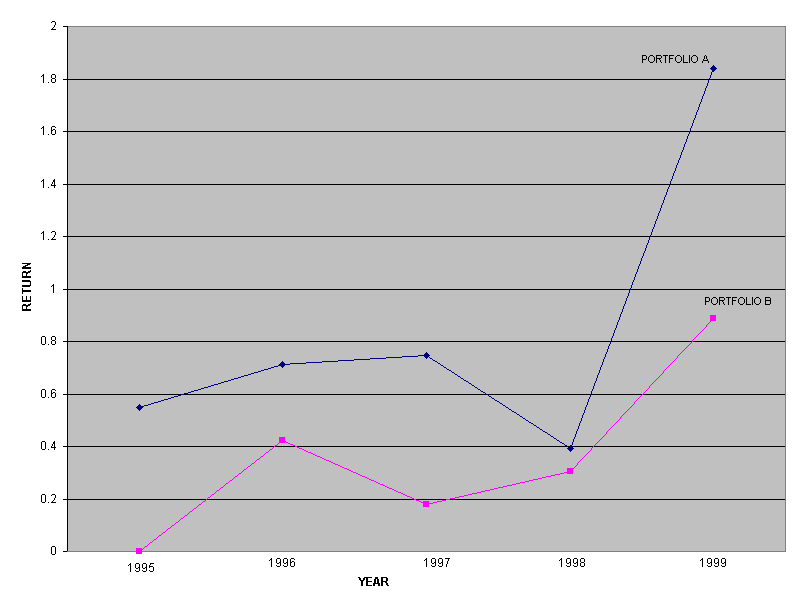
FIGURE 2: Mean Returns of Stocks in Asia/Pacific Portfolio A vs. Mean Returns of Stocks in Asia/Pacific Portfolio B by Year, 1995-1999

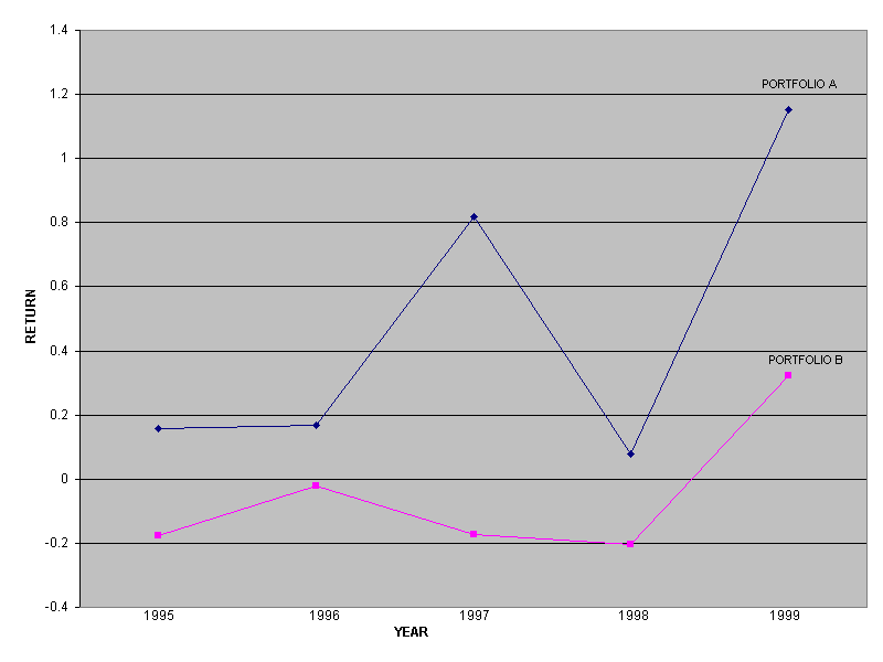
FIGURE 3: Mean Returns of Stocks in Europe Portfolio A vs. Mean Returns of Stocks in Europe Portfolio B by Year, 1995-1999

ENDNOTES

¹ The author is grateful for the contribution of Institutional Brokers Estimate System, Inc. for providing the earnings expectations data used in this study.

²Foreign currencies are converted to U S dollars based upon the exchange rates as of December 16 in each year, 1994-1999, complied in I/B/E/S database.

³Descriptive Statistics of SUE and Return for Europe Portfolios A1-A20 and B10-B20 are available upon request.

⁴The portfolios returns were extremely low in 1998 due to the currency crisis in Asia/Pacific that year.

SOURCES

1. Abarbanell, Jeffrey, and Victor Bernard. 1992. "Tests of Analysts' Overreaction/Underreaction to Earnings Information as an Explanation for Anomalous Stock Price Behavior." Journal of Finance (47:1181-1208).

2. Alexander, John C. Jr., and James S. Ang. 1998. "Do Equity Markets Respond to Earnings Paths?" Financial Analysts Journal (54: 81-94).

3. Amir, Eli, and Yoav Ganzach. 1998. "Overreaction and Underreaction in Analysts' Forecasts." Journal of Economic Behavior & Organization (37: 333-347).

4. Andreassen, Paul. 1990. "Judgmental Extrapolation and Market Overreaction: On the Use and Disuse of News." Journal of Behavioral Decision Making (3:153-174).

5. Bagnoli, Mark, Messod D. Beneish, and Susan G. Watts. 1999. "Whisper Forecasts of Quarterly Earnings Per Share." Journal of Accounting & Economics (28: 27-50).

6. Ball, Ray, and S. P. Kothari. 1989. "Non-Stationary Expected Returns: Implications for Tests of Market Efficiency and Serial Correlation in Returns." Journal of Financial Economics (25:51-74).

7. Bauman, W. Scott, C. Mitchell Conover, and Robert E. Miller. 1999. "Investor Overreaction in International Stock Markets." The Journal of Portfolio Management (25: 102-111).

8. Bernard, Victor.1993. "Stock Price Reactions to Earnings Announcements: A Summary of Recent Anomalous Evidence and Possible Explanations." In Advances in Behavioral Finance, edited by Richard H. Thaler, 303-340, New York: Russell Sage Foundation.

9. _____, and Jacob Thomas. 1989. "Post-Earnings Announcement Drift: Delayed Price Response or Risk Premium?" Journal of Accounting Research (27: 1-36).

10. _____. 1990. "Evidence That Stock Prices Do Not Fully Reflect the Implications of Current Earnings for Future Earnings." Journal of Accounting and Economics (13: 305-340).

11. Brous, Peter A., and Omesh Kini. 1993. "A Reexamination of Analysts Earnings Forecasts for Takeover Targets." Journal of Financial Economics (33:201-226).

12. Brown, Lawrence D. 1993. " Earnings Forecasting Research: Its Implications for Capital Markets Research." International Journal of Forecasting (9: 295-320).

13. Butler, Kirt C., and Larry H. Lang. 1991. "The Forecast Accuracy of Individual Analysts: Evidence of Systematic Optimism and Pessimism." Journal of Accounting Research (29: 150-156).

14. Carleton, Willard T., Carl R. Chen, and Thomas L. Steiner. 1998. "Optimism Biases among Brokerage and Non-brokerage Firms' Equity Recommendations: Agency Costs in the Investment Industry." Financial Management (27:17-30).

15. Charitou, Andreas, and George Panagiotides. 1999. "Financial Analysis, Future Earnings and Cash Flows, and the Prediction of Stock Return: Evidence for the UK." Accounting and Business Research (29: 281-298).

16. Cheung, Joseph K., Richard Chung, and Joeng-Bon Kim. 1997. "The Profitability of Trading Strategies Based on Book Value and Earnings in Hong Kong: Market Inefficiency vs. Risk Premia," Journal of International Financial Management & Accounting (8: 204-233).

17. Chopra, Navin, Josef Lakonishok, and Jay Ritter. 1993. "Measuring Abnormal Performance: Do Stocks Overreact?" In Advances in Behavioral Finance, edited by Richard H. Thaler, 265-302, New York: Russell Sage Foundation.

18. Chopra, Vijay Kumar. 1998. "Why So Much Error in Analysts' Earnings Forecasts?" Financial Analysts Journal (54: 35-42).

19. Clayman, Michelle, and Robin Schwartz. 1994. "Falling in Love Again - Analysts' Estimates and Reality." Financial Analysts Journal (50:66-68).

20. Daniel, Kent, David Hirshleifer, and Avanidhar Subrahmanyam. 1998. "Investor Psychology and Security Market Under- and Overreactions." Journal of Finance (53:1839-1885).

21. Das, S., C. B. Levine, and K. Sivaramakrishnan. 1998. "Earnings Predictability and Bias in Analysts' Earnings Forecasts." The Accounting Review (73: 277-294).

22. DeBondt, Werner F.M., and Richard Thaler. 1990. "Do Security Analysts Overreact?" American Economic Review (80:52-57).

23. Dreman, David N., and Michael A. Berry. 1995. "Analyst Forecasting Errors and Their Implications for Security Analysis." Financial Analysts Journal (51: 30-41).

24. Dugar, A., and S. Nathan. 1995. "The Effects of Investment Banking Relationships on Financial Analysts' Earnings Forecasts and Investment Recommendations." Contemporary Accounting Research 12:131-160.

25. Easterwood, John C. and Stacey R. Nutt. 1999. "Inefficiency in Analysts' Earnings Forecasts: Systematic Misreaction or Systematic Optimism?" Journal of Finance (54:1777-1797).

26. Fama, Eugene. 1970. "Efficient Capital Markets: A Review of Theory and Empirical Work." Journal of Finance (25:383-417).

27. _____. 1991. "Efficient Capital Markets: II." Journal of Finance 46:1575-1618.

28. _____. 1998. "Market Efficiency, Long-Term Returns, and Behavioral Finance." Journal of Financial Economics (49: 283-306).

29. Francis, Jennifer, and Donna Philbrick. 1993. "Analysts' Decisions as Products of a Multi-Task Environment." Journal of Accounting Research (31: 216-230).

30. Haugen, Robert A. 1999. The Inefficient Stock Market- What Pays Off and Why. Prentice Hall Inc., Upper Saddle River, New Jersey.

31. _____. 1999. The New Finance- The Case Against Efficient Markets. second edition, Prentice Hall Inc., Upper Saddle River, New Jersey.

32. Hayes, Rachel M. 1998. "The Impact of Trading Commission Incentives on Analysts' Stock Coverage Decisions and Earnings Forecasts." Journal of Accounting Research (36: 299-320).

33. Hunton, J. E., and R. A. McEwen. 1997. "An Assessment of the Relation Between Analysts' Earnings Forecast Accuracy, Motivational Incentives and Cognitive Information Search Strategy." The Accounting Review (72: 497-515).

34. Kang, Sok-Hyon, John O'Brien, and K. Sivaramakrishnan. 1994. "Analysts' Interim Earnings Forecasts: Evidence on the Forecasting Process." Journal of Accounting Research (32: 103-112).

35. Mendenhall, Richard. 1991."Evidence on the Possible Underweighting of Earnings-Related Information." Journal of Accounting Research (29: 170-179).

36. Lin, H., and M. F. McNichols. 1998. "Underwriting Relationships, Analysts' Earnings Forecasts and Investment Recommendations." Journal of Accounting and Economics (25:101-128).

37. Olsen, Robert. 1996. "Implications of Herding Behavior for Earnings Estimation, Risk Assessment, and Stock Returns." Financial Analysts Journal (52: 37-41).

38. Pratt, Tom. 1993. "Wall Street's four-Letter Word." Investment Dealers Digest (March: 18-22).

39. Schipper, K. 1991. "Commentary on Analyst Forecasts." Accounting Horizons (5: 105-121).

40. Shefrin, Hersh, 2000. Beyond Greed and Fear. Harvard Business School Press, Boston, Massachusetts.

41. Womack, Kent L. 1996. "Do Brokerage Analysts' Recommendations Have Investment Value?" Journal of Finance (51: 137-167).

Panel III. Asia/Pacific Portfolios A1-B20